Deep
Patterns
Hidden Patterns asked whether you could spot the algorithm. This asks whether you can build it, understand why it scales the way it does, and find it in the real world.
This will take several sessions. That's the point.
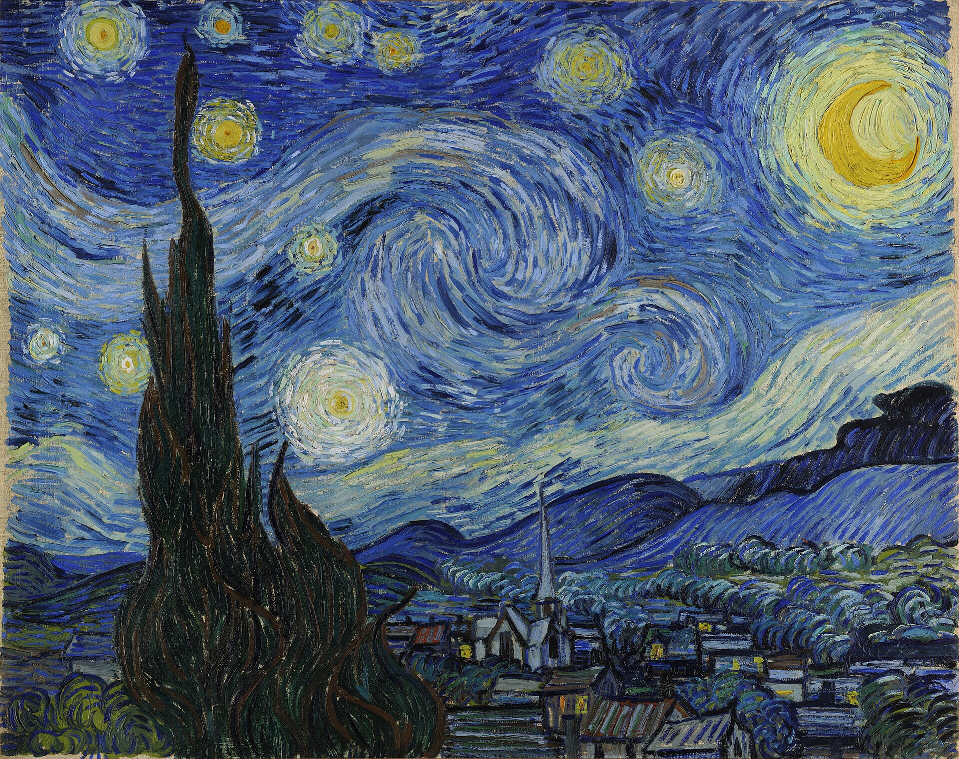
The Starry Night
B — The algorithm
Particles advected through a curl-noise flow field
Van Gogh's sky is not random. The brushstrokes follow coherent streamlines that swirl, split and rejoin — the visual signature of a vector field. We reproduce it by seeding thousands of massless particles and pushing each one along the local flow, frame after frame.
The field itself is the curl of a smooth scalar noise function. Taking the curl guarantees the flow is divergence-free — particles circulate rather than pile up — which is exactly why the result reads as turbulence rather than noise.
pt+1 = pt + (∇ × ψ)(pt) · Δt
Eq. 1 — explicit Euler advection step
# one frame — O(n), n particles, no interaction
for p in particles:
    vx, vy = curl(psi, p.x, p.y)
    p.x += vx * dt
    p.y += vy * dt
    if offscreen(p):
        reseed(p)   # keep density constant
C — The complexity
Linear — and that is the whole point
Each particle reads the field once and moves. No particle looks at any other. That independence makes one frame O(n) — double the particles, double the work, no worse. The table below contrasts that with the O(n²) cost you would pay if every particle had to consider every other, as a naïve fluid solver does.
| particles n | O(n) | O(n log n) | O(n²) naïve |
|---|---|---|---|
| 100 | 100 | 664 | 10,000 |
| 1,000 | 1,000 | 9,966 | 1,000,000 |
| 10,000 | 10,000 | 132,877 | 100,000,000 |
| 1,000,000 | 1,000,000 | 19,931,569 | 1,000,000,000,000 |
D — In the real world
Where linear flow fields earn their keep
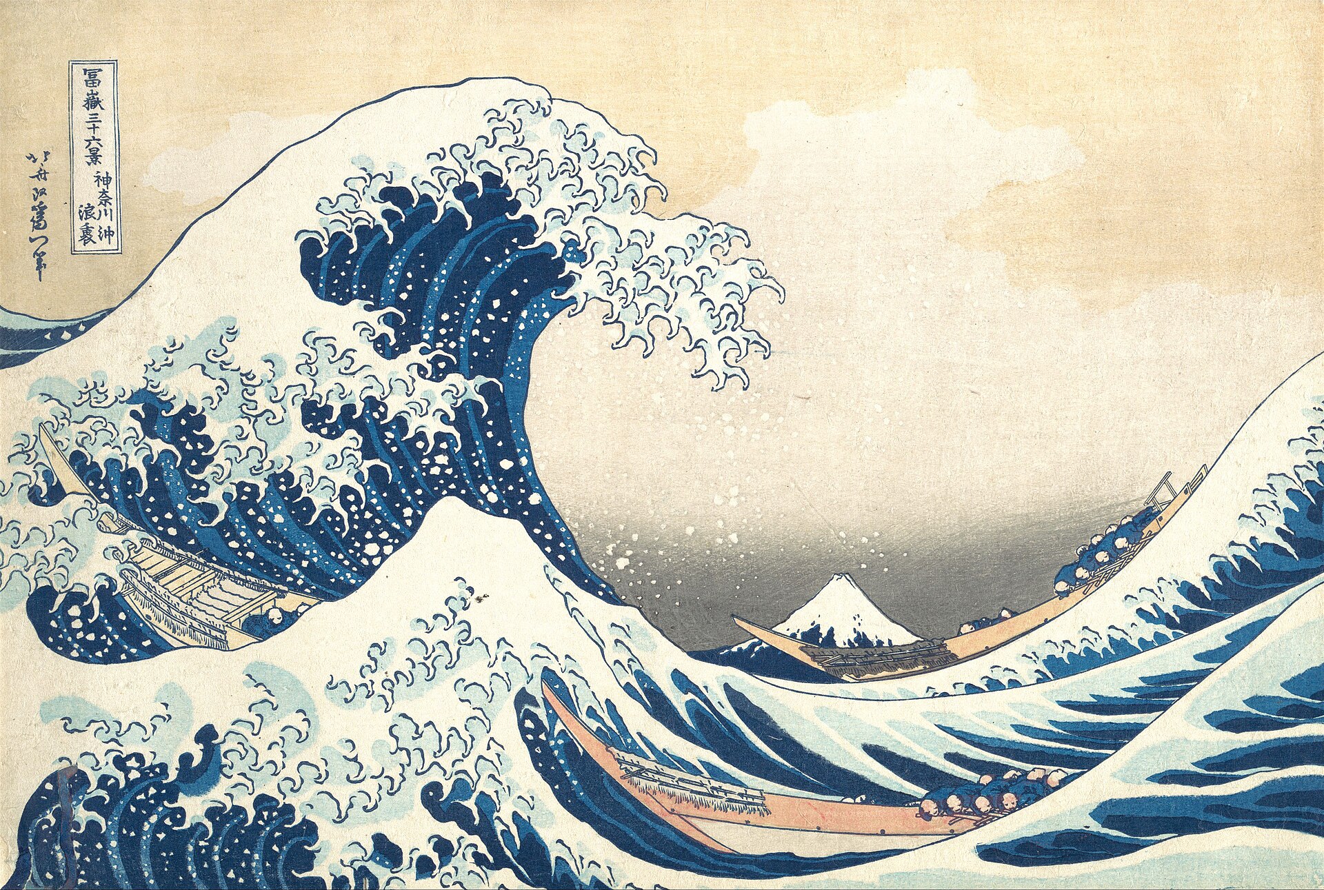
The Great Wave
B — The algorithm
A grid of heights evolving under the wave equation
Hokusai's wave captures the moment before a crest breaks — the peak of a travelling disturbance through water. The 2D wave equation describes how height disturbances propagate through a fluid surface at speed c. Each point in the grid depends only on its state at the two previous time steps and its four nearest neighbours.
Discretised with finite differences, this becomes an update rule that requires no matrix operations, no global solves. Each cell is independent; the wave emerges from the aggregate of local interactions.
∂²η/∂t² = c²∇²η
Eq. 1 — 2D wave equation (height η, speed c)
ηt+1 = 2ηt − ηt−1 + c²Δt²∇2hηt
Eq. 2 — explicit finite-difference (Verlet integration)
# one time step — O(n), n = grid cells
for y in range(1, H-1):
    for x in range(1, W-1):
        lap = (h[y,x-1] + h[y,x+1]
             + h[y-1,x] + h[y+1,x] - 4*h[y,x])
        h_next[y,x] = (2*h[y,x] - h_prev[y,x]
                     + c**2 * lap) * damping
h_prev, h, h_next = h, h_next, h_prev
C — The complexity
Linear updates — but an unsolved problem hides inside
The update rule above is O(n) per time step, where n is the number of grid cells. Double the grid, double the work. No surprises there.
But notice what we quietly skipped. The simulation uses a simplified wave equation — not the Navier-Stokes equations that govern real fluid dynamics. Those are different in kind: non-linear, fully coupled, and despite over 170 years of effort, not fully understood.
| grid cells n | O(n) | O(n log n) | O(n²) direct |
|---|---|---|---|
| 100 | 100 | 664 | 10,000 |
| 1,000 | 1,000 | 9,966 | 1,000,000 |
| 10,000 | 10,000 | 132,877 | 100,000,000 |
| 1,000,000 | 1,000,000 | 19,931,569 | 1,000,000,000,000 |
Clay Millennium Prize · $1,000,000
Navier–Stokes existence and smoothness
Given a smooth initial velocity field for a 3D incompressible fluid, do the Navier–Stokes equations have a smooth solution for all future time — or can they develop a singularity (a point where velocity becomes infinite) in finite time? The Clay Mathematics Institute designated this one of seven Millennium Prize Problems in the year 2000. It remains unsolved. Your simulation sidesteps the question by using a linear approximation. Real ocean-wave models do the same, for the same reason.
D — In the real world
Where wave equations earn their keep
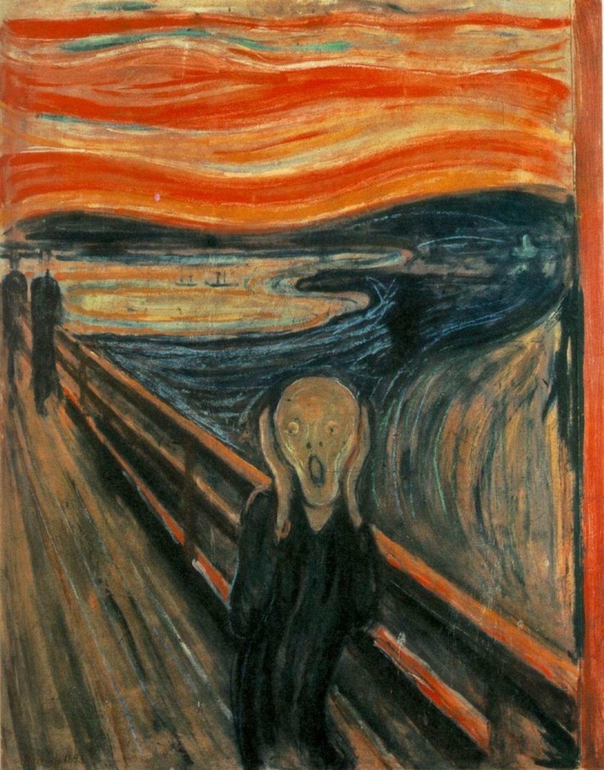
The Scream
B — The algorithm
Two chemicals, one unstable equilibrium, and Turing patterns
In 1952, Alan Turing — better known for his work on computation and codebreaking — published a paper arguing that certain chemical systems could spontaneously produce spatial patterns from a nearly uniform initial state. The turbulent sky of The Scream, with its swirling organisation, has something of this quality: a system driven from equilibrium, trying to arrange itself.
The Gray-Scott model captures the essence with two interacting chemicals U and V. U is fed in from outside at rate F. When U and V meet, they produce more V (autocatalytic reaction). V also decays at rate k. Crucially, the two diffuse at different rates — U fast, V slow. This asymmetry is the mechanism: V concentrates where it forms, while U replenishes the gaps, producing self-sustaining spatial structure.
∂u/∂t = Du∇²u − uv² + F(1−u)
∂v/∂t = Dv∇²v + uv² − (F+k)v
Eq. 1 — Gray-Scott reaction–diffusion model
# one Gray-Scott step — O(n), n = grid cells
for y in range(H):
    for x in range(W):
        lu = laplacian(u, x, y)   # 4-neighbour sum
        lv = laplacian(v, x, y)
        uvv = u[y,x] * v[y,x]**2  # autocatalytic term
        u_next[y,x] = u[y,x] + Du*lu - uvv + F*(1 - u[y,x])
        v_next[y,x] = v[y,x] + Dv*lv + uvv - (F+k)*v[y,x]
u, v = u_next, v_next
C — The complexity
Linear in space — but how long until the pattern?
The update rule is O(n) per step: each cell reads its four neighbours and applies a fixed formula. The table looks identical to the others. The interesting question is different: you cannot predict, from the initial conditions, how many steps will pass before a coherent pattern emerges.
The Gray-Scott system has a transient phase — a period of apparent disorder before the pattern crystallises. The length of that transient depends on F, k, and the initial perturbations in ways that resist analytical bounds. In biological contexts, this corresponds to the actual developmental timeline: a zebrafish's stripe pattern takes as long as it takes, regardless of how many cells are computing it.
| grid cells n | O(n) per step | O(n log n) | O(n²) naïve |
|---|---|---|---|
| 100 | 100 | 664 | 10,000 |
| 1,000 | 1,000 | 9,966 | 1,000,000 |
| 10,000 | 10,000 | 132,877 | 100,000,000 |
| 1,000,000 | 1,000,000 | 19,931,569 | 1,000,000,000,000 |
D — In the real world
Where reaction–diffusion shows up, uninvited
Downloads
Run it on your own machine
Open on a desktop to download and run the scripts.
# one-time setup
pip install numpy matplotlib

# run any script
python starry_night.py
python great_wave.py
python the_scream.py
Challenge progression · four tiers per painting
The Starry Night
The Great Wave
The Scream
About the scripts
Each script is a self-contained implementation of the algorithm from the browser page, written for readability not performance. The code matches the pseudocode in section B — you should recognise every line.
matplotlib's FuncAnimation handles the update loop. The simulation logic is separate from the display — you can swap in a different renderer without touching the physics.
Requires Python 3.9+ · numpy ≥ 1.22 · matplotlib ≥ 3.5